Transformations
All single-object transformations accept two possible syntaxes:
    transform(parameters, solid1, solid2, ...)
    transform(parameters) * solid1
The second, multiplicative form allows easy chaining of transformations:
transform1(param1) * transform2(param2) * solidThis form may also be applied to several solids by either wrapping them in a union, or equivalently, by applying it to a Vector of such objects:
transform(parameters) * [ solid1, solid2, ... ]Affine transformations
ConstructiveGeometry.mult_matrix — Functionmult_matrix(a, [center=c], solid...)
mult_matrix(a, b, solid...)
mult_matrix(a, b) * solid
a * solid + b # preferred formRepresents the affine operation x -> a*x + b.
Extended help
The precise type of parameters a and b is not specified. Usually, a will be a matrix and b a vector, but this is left open on purpose; for instance, a can be a scalar (for a scaling). Any types so that a * Vector + b is defined will be accepted.
Conversion to a matrix will be done when meshing.
Chained affine transformations are composed before applying to the objects. This saves time: multiple (3 × n) matrix multiplications are replaced by (3 × 3) multiplications, followed by a single (3 × n).
julia> s = mult_matrix([1 0 0;0 1 0;0 .5 1])*cube(10);
Only invertible affine transformations are supported. Transformations with a negative determinant reverse the object (either reverse the polygon loops, or reverse the triangular faces of meshes) to preserve orientation.
For non-invertible transformations, see project.
Three-dimensional embeddings of two-dimensional objects
As an exception, it is allowed to apply a (2d -> 3d) transformation to any two-dimensional object. The result of such a transformation is still two-dimensional (and will accordingly be rendered as a polygon), but the information about the embedding will be used when computing convex hull or Minkowski sum with a three-dimensional object.
julia> s = hull([30,0,0]+[1 0 0;0 1 0;.5 0 0]*circle(20), [0,0,30]);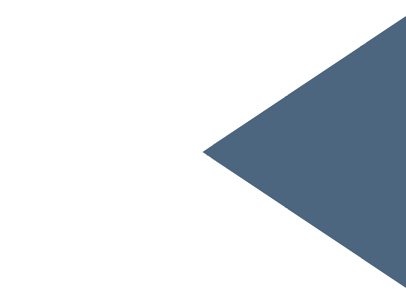
ConstructiveGeometry.translate — Functiontranslate(v, s...)
translate(v) * s
v + sTranslates object(s) s... by vector v.
ConstructiveGeometry.scale — Functionscale(a, s...; center=0)
scale(a; center=0) * s
a * sScales solids s by factor a. If center is given then this will be the invariant point.
a may also be a vector, in which case coordinates will be multiplied by the associated diagonal matrix.
julia> s = [1,1.5,2]*sphere(50);
ConstructiveGeometry.rotate — Functionrotate(θ, [center=center], [solid...])Rotation around the Z-axis (in trigonometric direction, i.e. counter-clockwise).
rotate(θ, axis=axis, [center=center], [solid...])Rotation around any axis, given by a vector directing this axis.
rotate((θ,φ,ψ), [center=center], [solid...])Rotation given by Euler angles (ZYX; same ordering as OpenSCAD).
Angles are in degrees by default. Angles in radians are supported through the use of Unitful.rad.
julia> s = rotate(30)*square(20);
ConstructiveGeometry.reflect — Functionreflect(v, s...; center=0)
reflect(v; center=0) * sReflection with axis given by the hyperplane normal to v. If center is given, then the affine hyperplane through this point will be used.
ConstructiveGeometry.raise — Functionraise(z, s...)For volumes: equivalent to translate([0,0,z], s...). For shapes: equivalent to translate([0,z], s...).
ConstructiveGeometry.lower — Functionlower(z, s...)For volumes: equivalent to translate([0,0,-z], s...). For shapes: equivalent to translate([0,z], s...).
Overloaded operators
The following operators are overloaded.
matrix * solidis a linear transformation.vector * solidis a multiplication by a diagonal matrix.vector + solidis a translation.real * solidis a scaling.complex * 2dshapeis a similitude.color * solidis acoloroperation.color % solidis ahighlightoperation.
Two-dimensional drawing
ConstructiveGeometry.offset — Functionoffset(r, solid...; kwargs...)
offset(r; kwargs...) * solidOffsets by given radius. Positive radius is outside the shape, negative radius is inside.
Parameters for 2d shapes:
ends=:round|:square|:butt|:loop
join=:round|:miter|:square
miter_limit=2.0
Parameter for 3d solids:
maxgrid = 32 # upper bound on the number of cubes used in one directionOffset of a volume is a costly operation; it is realized using a marching cubes algorithm on a grid defined by maxgrid. Thus, its complexity is cubic in the parameter maxgrid.
The grid size used for offsetting is derived from the atol and rtol parameters, and upper bounded by the optional maxgrid parameter (if this is different from zero).
julia> s1 = offset(10)*[square(100,50), square(50,100)];

julia> s2 = offset(3)*cube(30);

ConstructiveGeometry.opening — Functionopening(r, shape...; kwargs...)Morphological opening: offset(-r) followed by offset(r). Removes small appendages and rounds convex corners.
julia> s = opening(10)*[square(100,50), square(50,100)];
ConstructiveGeometry.closing — Functionclosing(r, shape...; kwargs...)Morphological closing: offset(r) followed by offset(-r). Removes small holes and rounds concave corners.
julia> s = closing(10)*[square(100,50), square(50,100)];
Extrusion
Prism (linear extrusion)
ConstructiveGeometry.prism — Functionprism(h, s...; twist, scale) # preferred form
prism(h; twist, scale) * s
linear_extrude(h, s...; twist, scale)
linear_extrude(h) * s...Build a prism (linear extrusion) of height h on the given base shape.
julia> s1 = prism(10)*[square(10,5), square(5,15)];


julia> s2 = prism(20, twist=45, scale=.8)*[square(10,5), square(5,15)];

Revolution (rotational extrusion)
ConstructiveGeometry.revolution — Functionrevolution([angle = 360°], shape...; slide=0)
revolution([angle = 360°]; [slide=0]) * shape
rotate_extrude([angle = 360°], shape...; slide=0)
rotate_extrude([angle = 360°]; [slide=0]) * shapeSimilar to OpenSCAD's rotatre_extrude primitive.
The slide parameter is a displacement along the z direction.
julia> s1 = revolution(245)*[square(10,5), square(5,15)];


julia> s2 = revolution(720, slide=30)*translate([10,0])*square(5);

The number of samples used for a revolution depends on the radius (i.e. the maximal abscisssa of a point on the shape) and the atol and rtol parameters, in the same way as the number of vertices of a circle does; see Number of vertices of circles.
Conical extrusion
The cone function may also be used as an operator to build a cone out of an arbitrary shape:
julia> s = cone([1,2,3])*square(5);
Surface sweep
ConstructiveGeometry.sweep — Functionsweep(path, shape...)Extrudes the given shape by
- rotating perpendicular to the path (rotating the unit y-vector to the direction z), and
- sweeping it along the
path, with the origin on the path.
sweep(transform, volume)Sweeps the given volume by applying the transform:
V' = ⋃ { f(t) ⋅ V | t ∈ [0,1] }
f is a function mapping a real number in [0,1] to a pair (matrix, vector) defining an affine transform.
- nsteps: upper bound on the number of steps for subdividing the [0,1] interval
- gridsize: subdivision for marching cubes
- isolevel: optional distance to add/subtract from swept volume
Extended help
The sweep feature currently has two main limitations:
- the trajectory may only contain closed loops (no open paths);
- the extrusion of each profile vertex must preserve this topology.
Both of these restrictions are due to the clipper library, which does not support single-side offset. For an (experimental) remedy, see path_extrude.
Volume sweep is a costly operation, implemented using a marching cubes algorithm on a grid defined by gridsize. Thus, its complexity is cubic in the parameter gridsize.
FIXME: unify gridsize and offset's maxgrid parameters.
A swept surface is similar to a (closed) path extrusion:
julia> s = sweep(square(50))*circle(5);
julia> f(t) =([ cospi(t) -sinpi(t) 0;sinpi(t) cospi(t) 0;0 0 1],[0 0 10*t]);

julia> s = sweep(f; nsteps=100,maxgrid=100)*cube(20);
Path extrusion
ConstructiveGeometry.path_extrude — Functionpath_extrude(trajectory)*profileExtrusion of the given profile along the trajectory.
This feature is still experimental. Success is not guaranteed. Also, API should not be considered stable.
julia> s = path_extrude([[[0,0.],[3,0],[5,1]]])*(square(10)-([1,2]+square([6,5])));
[1;7m before splitting segments:[m
Input mesh is not PWN!
User-defined volume deformations
ConstructiveGeometry.deform — Functiondeform(f, s...; isvalid, distance2)Image of the volume s by the vertex-wise transformation f (as a function on SVector{3} points).
After applying the transformation, overlapping parts of the volume are cleaned by a self-union operation. It is however the user's responsibility to ensure that the image still forms a valid, positively-oriented mesh.
Since f is (in principle) not a linear function, all edges longer than the the current atol meshing parameter will be split, using the refine transformation, before applying f to the vertices.
Optional parameters:
isvalid: a predicate which will be asserted on all points of the solid before applying the transformation;distance2: a function for evaluating which edges should be split. The default is to use the Euclidean distance.
julia> s1 = deform(p->p/(3+p[1]))*cube(5);

julia> s2 = deform(p->p/sqrt(1+p[1]))*cube(5);

Cylindrical wrapping (experimental)
ConstructiveGeometry.wrap — Functionwrap(r, s...)Wraps the solid s around a cylinder with radius r by applying the coordinate transformation $(x \cos(y/r), x \sin(y/r), z)$. Long edges will be split so that their image resembles the correct spirals.
julia> s = wrap(3)*cube(5);
Decimation
These operations either reduce or increase the number of faces in a three-dimensional object.
ConstructiveGeometry.decimate — Functiondecimate(n, surface...)Decimates a 3d surface to at most n triangular faces.
ConstructiveGeometry.loop_subdivide — Functionloop_subdivide(n, shape...)Applies n iterations of loop subdivision to the solid. This does not preserve shape; instead, it tends to “round out” the solid.
julia> s = loop_subdivide(4)*cube(20);
ConstructiveGeometry.refine — Functionrefine(maxlen, volume...)Splits all edges of volume repeatedly (preserving global geometry), until no edge is longer than maxlen.
Coloring objects
ConstructiveGeometry.color — Functioncolor(c::Colorant, s...)
color(c::AbstractString, s...)
color(c::AbstractString, α::Real, s...)
color(c) * s...
colorant"color" * s...Colors objects s... in the given color.
julia> green, red = colorant"green", colorant"red"
(RGB{N0f8}(0.0,0.502,0.0), RGB{N0f8}(1.0,0.0,0.0))

julia> s = union(green * cube(10), [10,0,0]+red*sphere(10));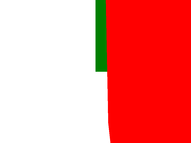
Highlight
ConstructiveGeometry.highlight — Functionhighlight(c::Colorant, s)
highlight(c::AbstractString, s)
(c::Colorant) % sMarks an object as highlighted. This means that the base object will be displayed (in the specified color) at the same time as all results of operations built from this object.
julia> s = intersect(green % cube(10), red % ([10,0,0]+sphere(10)));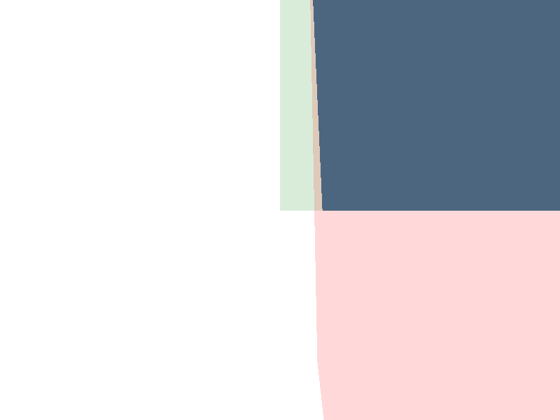
Highlighted parts of objects are shown only when the object is represented as an image via the plot method. For SVG and STL output, all highlighted parts are ignored.
Highlighted objects are preserved only by CSG operations and (invertible) affine transformations. For other transformations:
- convex hull and Minkowski sum are generally increasing transformations, and would cover highlighted parts anyway;
- projection, slicing and extrusion modify the dimension of object, making it impossible to preserve highlighted parts.
ConstructiveGeometry.randomcolor — Functionrandomcolor(s...)Paints each triangle of s in a random color. Intended for debugging purposes.
julia> s = randomcolor()*sphere(5);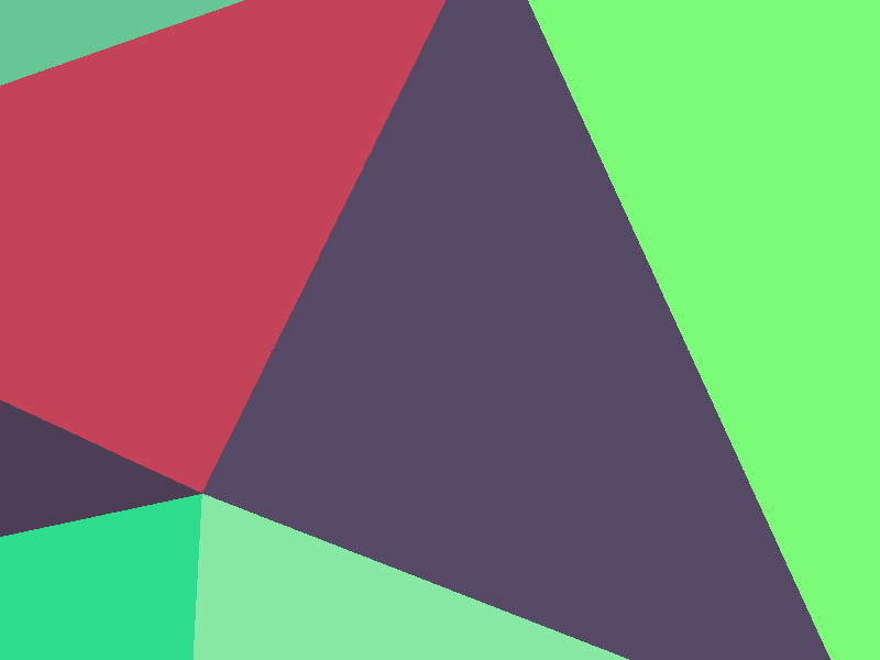
Modifying meshing parameters
ConstructiveGeometry.set_parameters — Functionset_parameters(;atol, rtol, symmetry, icosphere) * solid...A transformation which passes down the specified parameter values to its child. Roughly similar to setting $fs and $fa in OpenSCAD.
See meshing.md for documentation about specific parameters.
The set_parameters transformation allows attaching arbitrary metadata. This is on purpose (although there currently exists no easy way for an user to recover these metadata while meshing an object).
The values for these parameters are explained in atol and rtol.